INDEX(MATCH) function
If you've ever tried to match data from different sheets in the past, you've probably come across the VLOOKUP. The VLOOKUP is good for linking data from another sheet if you can influence the data to be linked. The search criterion must come first and the list must be sorted by the search criterion.
Sometimes it is not possible to prepare the data from the linked list for the VLOOKUP, as this would make the original list unusable. To enable an assignment in these cases as well, we use the INDEX and MATCH functions.
We first start with an explanation of the INDEX function:
=INDEX( matrix ; row ; if necessary column )

Since the function only returns a value from a matrix, but does not search the matrix itself, we combine it with the function MATCH:
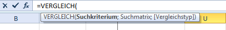
=MATCH( search_criterion ; matrix ; match type )
The function parameters already speak for themselves how the two functions are linked together (descriptive texts here for better understanding):
=INDEX(column from which we want to return a value;MATCH(current table[search_criterion];linked table[search_criterion];0))
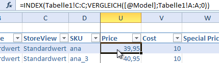
Applied to the example from How to use VLOOKUP to assign data we open the manufacturer list and load the products via cobby. Then we select the cell to which we want to transfer data from the manufacturer list (here: Price) and switch to the formula bar.
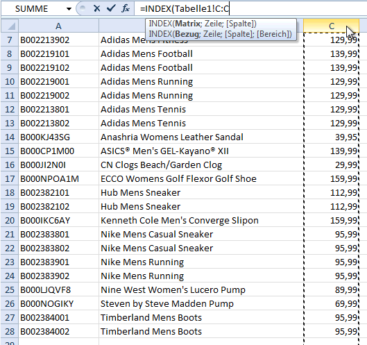
There we enter the formula for the INDEX =INDEX( .

Then we switch to the manufacturer list and click on the column header whose data we want to take over (here: Price column C).
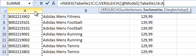
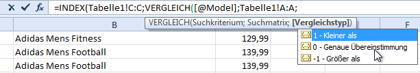
Now we enter a semicolon ( ; ) followed by the formula MATCH(. The first parameter for the function MATCH is the search criterion from our cobby sheet (here: Model, often EAN).

The second parameter tells the MATCH what to compare with. In this case, this is the Model column from the manufacturer list.
With another semicolon ( ; ) we still indicate that an exact match must be found. The constant for this is 0.
With two closed brackets )) we end the input of the formula and can now apply it by copy and paste or double click on the small rectangle in the cell for the whole column.